计算LD decay(LD衰减)

这次是介绍如何计算LD，并作出LD decay plot。

首先推荐一篇文献，作者们都是男神。

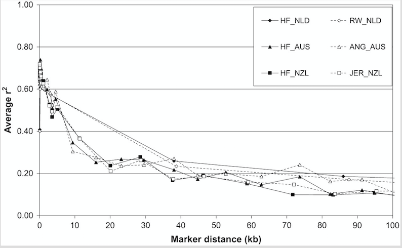
Linkage Disequilibrium and Persistence of Phase in Holstein-Friesian jersey and Angus Cattle, Roos et al. Genetics(2008)

文章中关于LD的概念，LD的计算方法，如何用LD推断Ne（有效群体大小）以及persistence of LD都讲得清楚。作出类似Figure1的图是本篇的主要目的。

衡量LD主要有D’和r2两个统计量，D’受到位点频率的影响，因而不如r2稳健。一般地，用r2来衡量位点之间LD的大小。 plink1.07 虽然提供了--r2命令来计算位点之间的连锁关系，但是这个命令的解释也说了“this calculates for each SNP the correlation between two variables, coded 0,1 or 2 to represent the number of non-reference alleles at each. The squared correlation based on genotypic allele counts is therefore not identical to the r-sq as estimated from haplotype frequencies, although it will typically be very similar.” 因而不推荐用此方法计算LD。

LD的r2值可以由Haploview软件完成。Haploview除了提供图形界面操作，还可以用命令行运行。计算r2的命令行如下：

java -jar Haploview.jar -nogui -pedfile example.ped -info example.info -dprime

生成的example.ped.ld文件中则包括了r2，格式如下所示。 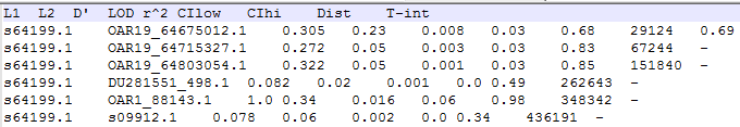这里的计算忽略了长度超过500kb的LD，如需修改可参考Haploview的帮助文档.

example.ped和example.info文件可以由plink软件转换，plink --bfile example --recodeHV --out example，则生成ped和info格式。

接下来是划定物理距离的间隔计算区间，计算某段物理位置之内的LD平均值，用以代表该物理位置的LD水平，所以，划定的区间不宜过大。

df<- read.table( "example.ped.ld",header=T)[,c(5,8)] #读取LD值
dist<- c(seq(0,100000,5000)) #计算0-100kb之间的LD衰减，每隔5kb计算一次LD平均值
#定义计算LD均值公式
ld_avg<- function(ld,dist) {
	ld_out<-c()
	for (i in 1:(length(dist)-1)){
	index<-(ld[,2]< dist[i+1])&(ld[,2]>dist[i])
	ld_out[i]<-mean(ld[index,1])
	}
	ld_decay<-cbind(ld_out,dist[-1])
	return(ld_decay)
}
#计算example.ped.ld 的平均LD
example_LDdecay <- ld_avg(df,dist)
#作图
png("example_ldDecay.png")
plot(example_LDdecay[,2],example_LDdecay[,1])
dev.off()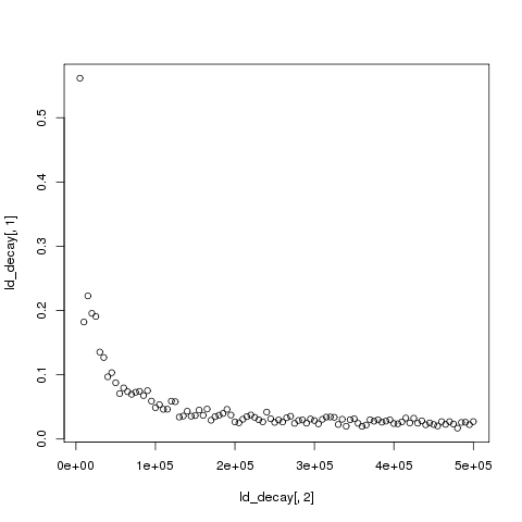

至此，做出了单条染色体的LD衰减图。若要计算全基因组水平的LD decay，可以先分别计算每一条染色体上标记之间的LD水平，将全部染色体的数据合并为一个文件，再用滑窗方式计算所划分的区间内的平均LD值，再作图即可。

假设通过Haploview软件，分别得到每条常染色体上的LD结果，文件名为chr1.ped.ld，chr2.ped.ld，chr3.ped.ld，chr4.ped.ld，… 合并所有的文件为同一个文件，chroms.ld，可以使用R中的rbind函数，或者利用shell，

awk 1 chr*ped.ld | sed '/T-int/d' >chroms.ld