利用PLINK进行GWAS分析(四)
IBS clustering 和 MDS
#IBS和IBD IBS, Identity by State</br> IBD, Identity by Descent</br>
Wikipedia对IBD,IBS的解释</br>
A DNA segment is identical by state (IBS) in two or more individuals if they have identical nucleotide sequences in this segment. An IBS segemet is identical by descent (IBD) in two or more individuals if they have inherited it from a common ancestor without recombination, that is, the segment has the same ancestral origin in these individuals. DNA segments that are IBD are IBS per definition, but segments that are not IBD can still be IBS due to the same mutations in different individuals or recombinations that do not alter the segment.</br>
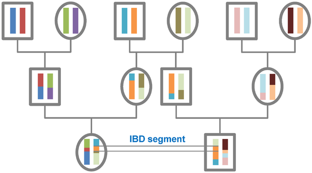
简单来说,两个个体都含有相同基因序列的DNA片段,这一DNA片段肯定是IBS,如果这一DNA片段是遗传自同一个共同祖先,那么这一DNA片段也是IBD。</br>
比较两个个体之间的SNP的Identity by State,分为三个状态:</br> 1、Identical,完全一致。如果在两个个体中都是相同基因型,AA & AA,AB & AB或者BB & BB。</br> 2、One-Allele Shared,含有一个共同位点。比如两个个体基因型为AA & AB或者BB & AB。</br> 3、No alleles shared,没有共同位点。比如,AA & BB。</br> 因而根据IBS对个体的基因型编码,这三种IBS状态可以相应地编码为2,1,0。即含有两个相同位点,含有一个相同位点,没有相同位点。</br>
简单理解,基因组上含有相同DNA片段越多的两个个体间的亲缘关系越近。</br> IBD和IBS都可以用来推断个体之间的遗传亲缘关系。 参考文献:Stevens et al. 2011. Inference of Relationships in Population Data Using Identity-by-Descent and Identity-by-State.PLoS Genet 7(9):e1002287</br>
需要有家系等额外的信息才能够判断IBD。因而对于一般的随机抽样群体,没有系谱记录的话,用IBS判断亲缘关系远近。</br>
PLINK计算群体中两两个体之间的IBS,构成的是IBS得矩阵形式。
plink --file test --cluster --matrix
#生成plink.mibs,是两两个体间的IBS矩阵。数值在0~1之间,数值越小代表个体间相似度越低,亲缘关系越远
#Multidimensional scaling plots(MDS) 实际上是多维变量分解IBS矩阵。这里的MDS和PCA是一样的。关于MDS和PCA的原理和细节下次再叙述,这里主要说明如何生成MDS结果。
plink --file test --cluster --mds-plot 10
#生成plink.mds,这一文件从第四列开始,分别为第一、第二……的dimension。
plink.mds文件中每一行是一个个体的数据。
column1 = FamilyID
column2 = IndividualID
column3 = SOL, Assighed solution code
column4 = C1, Position on first dimension
column5 = C2, Position on second dimension
column6 = C3, Position on third dimension
column7 = C4, Position on fourth dimension
…………
根据第一和第二维度(第四列和第五列)的数据,绘制scatter plot,可以看到不同个体的在这两个维度上的坐标。
dat <- read.table ( "plink.mds", header = T)
pop <- dat[ ,1]
mds1 <- dat[ ,4]
mds2 <- dat[ ,5]
plot (mds1, mds2, col = as.factor(pop), xlab = "C1", ylab = "C2", pch = 20, main = "MDS plot")
legend("bottomleft", bty = "n", cex = 0.8, legend = unique(pop), border = F, fill = unique(as.factor(pop)))
#加上图注,并以第一列的FamilyID对个体标记不同的颜色。